Mapping Text to Knowledge Graph Entities using Multi-Sense LSTMs
Paper-ArXiv
Authors: Dimitri Kartsaklis, Mohammad Taher Pilehvar, Nigel Collier (University of Cambridge)
Venue: EMNLP 2018
Hypothesis
- Many KBs are sparse (lacking connections between many entities). Extending a KB using additional contexutal features can enrich them and connect the missing dots.
- This extended KB can be leveraged to create a synthetic corpus on which skipgram models can be trained to learn entity embeddings.
- To map text to entities in this KB, one needs to consider multiple senses associated with words in the text. To do this, one can use an LSTM whose input is the weighted averaged senses of words in the text (calculated by attention w.r.t context of the words).
Task
Mapping a textual description to KB entities (e.g., “can’t sleep, too tired to think straight” -> “Insomnia”) (also called grounding or normalization)
Model
- How to embed entities?
- Use a set of reliable anchors or textual features that would link entities with textual descriptions.
- The textual features are textual descriptions of the entity weighted by tf-idf values.
- Tf-idf values are computed by considering word frequencies in a document composed of textual descriptions of an entity (tf) against all other documents (df).
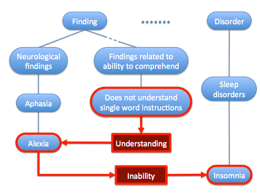
The blue nodes show the KB (SNOMED) and relationships between concepts/entities. The KB is further extended using words in textual descriptions corresponding to the blue entities. These are shown in red nodes. The edges are weighted according to the tf-idf values of the words in the textual descriptions of a given entity. This helps connecting entities that would not be otherwise connected. For example, here, *Alexia* and *Insomnia* both correspond to *inability* to something and therefore there could be some functional similarities between them. - After extending the KB, the entities are embedded using skip-gram model trained on a synthetic corpus build by random work on this extended KB.
- The random walk is done according to a distribution of either choosing the next entity (blue node) or next textual feature (red node).
- The textual features are textual descriptions of the entity weighted by tf-idf values.
- Use a set of reliable anchors or textual features that would link entities with textual descriptions.
- Text-to-entity mapping: Transformation from a textual vector space to a KB vector space.
- An LSTM encodes a sentence (description of the entity) into a point in the embedding space.
- The authors raise the issue of polysemy (words with slightly different meanings). As an example, while the lemma for the word “fever” in a dictionary usually contains two or three definitions, the term occurs in many dozens of different forms and contexts in SNOMED.
- They try to address this by extending a standard LSTM with a so called multi-sense LSTM that considers multiple sense-vectors given context in training.
- Each word is associated with a single generic embedding and $k$ sense embeddings.
- For each word $w_i$, a context vector $c_i$ is computed as the average of the generic vectors for all other words in the sentence.
- The probability of each sense vector $s_j$ given this context $c_i$ is then calculated via attention (capturing similarity between the context and the sense) \(p(s_j|c_i) = \frac{exp(\tanh(Ws_j+Uc_i))}{\sum_{l=1}^k exp(\tanh(Ws_l, c_8))}\)
- Each sense vector $s_i$ is updated by addition of the context vector weighted by its similarity with the specific sense. \(s_i = s_i + (s_i c_i) c_i\)
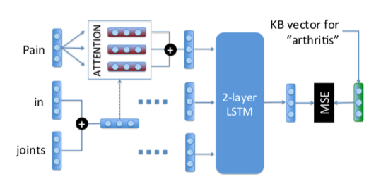
Green vector (on right) is the target vector in the KB and red vectors (on top left) are vectors corresponding to senses. The objective is to minimize the loss between the predicted vectors and the target vectors prepared using skip-gram model. Intuitively, the multi-sense LSTM computes a weighted average of the senses that are computed according to the similarity of the given word sense w.r.t to the context (average of other words in the sentence). In other words, the authors see what sense of the word is more appropriate in this context and then use it to calculate the sense embeddings. The weighted average of sense embeddings is then fed to an LSTM an results in a vector that predicts the entity.
- An LSTM encodes a sentence (description of the entity) into a point in the embedding space.
Results
- Evaluation is done on three tasks
- Text to entity mapping
-
A dataset of size 21,000 constructed from SNOMED concepts associated with multi-word textual descriptions.
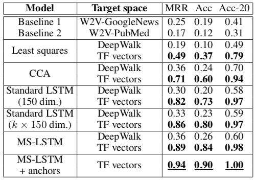
In Baselines 1 and 2 a vector for each textual description is computed as the average of pre-computed word vectors, and compared to concept vectors prepared in a similar way, i.e. by averaging pre-computed vectors for all words in the qualified name of the entities. In Least squares and CCA, an averaged vector for each textual description is again computed as before, and a linear mapping is learned between the textual space and the KB space, using least squares and canonical correlation analysis. The last row of the table presents results after extending the training dataset with the textual anchors, that is, all the textual features paired with their learned KB vectors. Specifically, recall that each textual feature (a word or), being also a node in the graph, is associated with a vector according to the process of §3.1. It is possible for one then to use these (textual feature, vector) pairs as additional examples during the training of the MS-LSTM.
-
- Reverse dictionary
- Dataset from WordNet by Hill et al (2016) where the goal is to return a word given its definition. Their method achieves up to 0.96 Acc-10 results a 3 point improvement over the best baseline.
- Document classification
- Cora (2078 papers with 7 categories)
- They achieve up to 88% accuracy a 1% improvement over the best baseline.
- Text to entity mapping
conclusions
Using a graph embedding space as a target for mapping text to entities is an effective approach.